Statistical Process Control (SPC) for Non-Statisticians
Statistical process control for managers: common and special causes, a run chart, then an XmR chart with limits worked out on 21 days of help-desk data.

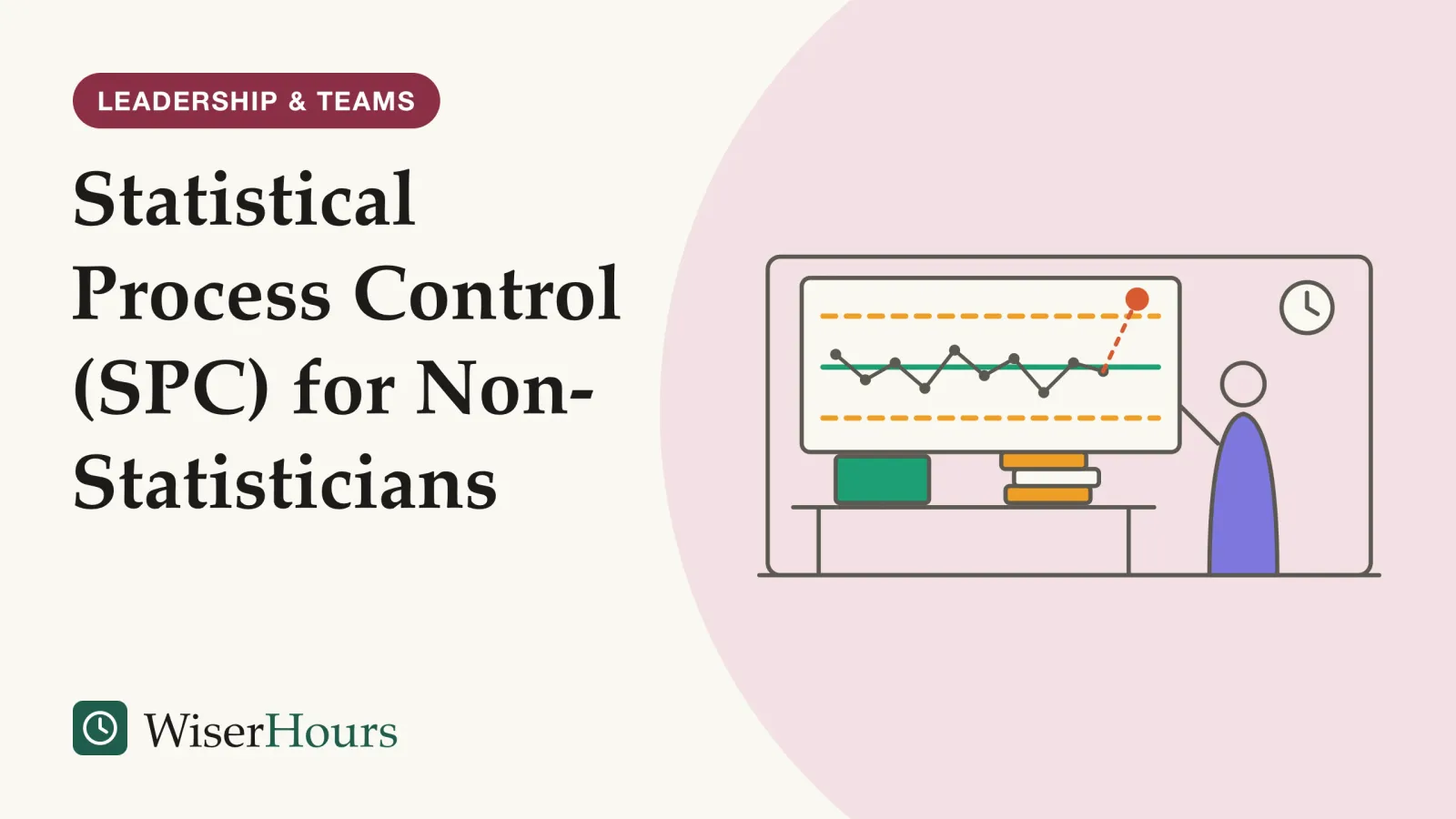
A help desk’s daily report shows the average time to resolve a ticket rising from 7 hours on Monday to 10 on Tuesday, and someone asks what went wrong. Often nothing did. Statistical process control (SPC) plots a measure in time order, with a center line and two limits worked out from the data, so a team can tell routine ups and downs from a change worth investigating. NHS England’s Making Data Count guide describes it as a way to understand variation and choose the right action.1
SPC is one of the measuring habits behind process improvement, and a natural fit for the control phase that closes every Six Sigma project. It needs no statistics degree: a spreadsheet, a few averages and one multiplication. The whole method fits in four moves. Plot the numbers in time order, find their average, set limits at the average plus and minus 2.66 times the average gap between neighboring points, and look into only the points that break a rule you agreed in advance.
Statistical process control in plain words
Statistical process control is a way of judging whether a process behaves consistently by plotting one measure over time against a center line and two control limits calculated from its own variation. Points inside the limits are routine; a point outside them suggests an assignable cause worth looking for, according to the NIST/SEMATECH e-Handbook of Statistical Methods, which NIST, the US federal standards agency, publishes online.2
Definition
Statistical process control (SPC) uses charts that plot a measure in time order, with limits calculated from the measure’s own variation, to tell routine variation from signs that the process has changed.
The idea comes from Walter Shewhart, who introduced the control chart in a one-page memo at Bell Labs in 1924. By then the company’s engineers had noticed that constantly adjusting a process whenever a part failed inspection made the variation worse.3 Shewhart’s name turns up again in the origins of the PDSA improvement cycle, a separate story.
The method answers a question that comparing two numbers cannot. Monday against Tuesday tells you nothing about how much the measure moves in an ordinary week. Most day-to-day movement in a stable process is routine variation, and the chart shows how big that routine movement is. Before asking why a number rose, ask whether it rose by more than usual.
Common-cause and special-cause variation
Common-cause variation is the ordinary spread a process produces every day; special-cause variation comes from something unusual that is not part of the process all the time. NHS England’s guide uses a commute: traffic and lift queues make the trip vary daily, while a broken-down train makes you an hour late.1
The two call for different responses. Common-cause variation belongs to the whole system, so it shrinks only when someone changes the system: staffing, ticket routing, training or tools. Chasing the reason for one ordinary bad day is what the NHS guide calls a wild goose chase, or tampering. A special cause can be found and dealt with: removed if it hurt, and, if it helped, learned from and kept.1
On a help desk, common causes include the daily mix of ticket types, who is on shift and the Monday backlog. A password system outage, a software release or a new team member’s first week are candidates for special causes.
The chart decides which kind you are looking at, so save the question “what was different about that day?” for points the chart flags.
Start with a run chart
A run chart is the simplest SPC tool: plot the measure in time order and draw a line at the medianmedian: The middle value when numbers are put in order, so half fall below it and half above. Unlike the average (mean), it is not pulled up or down by a few very large or very small values, which is why it is often used for incomes and wealth.Full entry in the glossary. The Institute for Healthcare Improvement (IHI) teaches four rules for reading one: a shift, a trend, too many or too few runs, and an astronomical point.4
The rules are counting rules, which is why they need no formulas. In IHI’s version, a shift is six or more points in a row on one side of the median, and a trend is five or more points in a row going up or down. Too many or too few runs (groups of points on one side) is checked against a reference table, and an astronomical point is an obvious outlier spotted by eye. The transcript is also blunt that two data points do not make a trend.4
NHS England’s guide suggests a run chart when you have fewer than 20 points, and certainly fewer than 10, then converting to a control chart once there are enough.1 A new help-desk lead with two weeks of daily figures can plot them, mark the median and read the four rules on the first afternoon.
Three bad days in a row on a run chart are worth noting, but under these rules they are not yet evidence that anything changed.
How to calculate control limits on an XmR chart
For one number per day, week or month, the chart to use is the XmR, or individuals, chart. Its center line is the average, and its limits sit 2.66 average moving ranges either side; a moving range is the gap between a point and the one before it. The NIST handbook writes the same formula as three times the average moving range divided by 1.128.5
NHS England’s guide suggests new users start with the XmR chart, which it calls the Swiss army knife of SPC charts because it is simple to build and explain.1 A 1997 Quality Digest column by Donald Wheeler gives the same 2.66 factor, plus 3.268 for the limit on the moving ranges themselves.6
The worked example below uses invented data: a help desk’s average resolution time for each of 21 working days, in hours.
| Step | What to do | Help-desk example |
|---|---|---|
| 1. Collect | One value per period, in time order | 10, 7, 7, 8, 8, 8, 9, 6, 8, 7, 9, 9, 10, 6, 10, 10, 7, 6, 8, 7, 8 |
| 2. Center line | Average all the values | 168 ÷ 21 = 8 hours |
| 3. Moving ranges | Subtract each value from the one before and drop the minus sign | 3, 0, 1, 0, 0, 1, 3, 2, 1, 2, 0, 1, 4, 4, 0, 3, 1, 2, 1, 1 |
| 4. Average moving range | Average the 20 ranges | 30 ÷ 20 = 1.5 hours |
| 5. Control limits | Average plus and minus 2.66 × average moving range | 8 ± 4.0: limits at 4 and 12 hours 5 |
| 6. Range limit | 3.268 × average moving range | About 4.9 hours; no range exceeds it 6 |
- Center line: the average of the 21 days, 8 hours
- Control limits: the average plus and minus 2.66 times the average moving range of 1.5 hours: about 4 and 12 hours
- A signal: a day above the upper limit (a hypothetical 13 hours) is worth investigating; the points inside the limits are routine variation
Every one of the 21 days falls between 4 and 12 hours, so this help desk is stable: its resolution time is predictable within that band. A 10-hour Tuesday is part of its normal week. If day 22 came in at 13 hours, above the upper limit, that would be a signal, and a good moment for a short root cause analysis.
One shortcut breaks the method. The same column shows that limits built from the standard deviationstandard deviation: A measure of how widely values spread around their average: small when most values sit close to it, large when they are scattered. Effect sizes are often given in standard deviations so that results measured on different scales can be compared.Full entry in the glossary of all the data, the figure a spreadsheet’s standard deviation function gives, come out too wide when the data contain signals, and so hide the very changes you are looking for. Limits built from moving ranges do not have that flaw.6 Use the moving-range formula, whatever the spreadsheet offers.
Reading the chart: four signal rules
Most teams need only a few agreed rules, because without them one person sees a clear change and another sees none. NHS England’s guide uses four: one point outside a limit, a run of points on one side of the center line, six points in a row rising or falling, and two out of three points close to a limit, in the outer third of the band.1
For the run rule, the guide says most people use seven to nine points, never fewer than six, and that teams with daily data may choose a longer run to avoid reacting too often.1 The NIST handbook lists a similar set, the Western Electric rules, which flag eight points in a row on one side.7 The exact numbers matter less than agreeing on them before anyone looks at the chart.
Every rule also raises false alarms now and then. With limits at three standard deviations and normally distributed data, a stable process puts a point outside the limits about once in every 370 points, according to Wikipedia’s summary of Wheeler’s figures.3 On a daily chart with about 250 working days a year, that is roughly one false alarm every year and a half, so adding many extra rules buys sensitivity at the price of more needless investigations.
How control limits differ from targets and specification limits
Control limits describe what the process does; targets and specification limits describe what someone wants it to do. The NIST handbook draws the line simply: control limits show whether a process is producing consistent output, while specification limits show whether the product will work as intended.7
Nobody sets control limits. They come from the data, and about 99 percent of points from a stable process fall inside them, according to NHS England’s guide.1
Where the target sits tells you what to expect. NHS England’s guide explains that a target outside the limits cannot be expected to be met without changing the process, while a target inside them will be met some periods and missed in others, so a red-amber-green report flips between red and green.1 Suppose the help desk is told to keep the daily average under 10 hours. That target falls inside its 4-to-12-hour band, so it will miss on some days with nothing wrong; hitting it every day needs a change to the system, such as better routing of ticket types.
- Myth
- The control limits are the range the team should aim for.
- Fact
- Control limits are calculated from the data and describe current performance. A target is a separate line you add to compare against it.
Draw the target in a different color from the limits, and read a missed target inside the limits as a reason to improve the system rather than to blame the day.
Why reacting to every point makes things worse
Adjusting a stable process after each result, in response to routine variation, makes its results more variable. W. Edwards Deming called this tampering and demonstrated it with his funnel experiment, in which marbles are dropped through a funnel aimed at a target, as a University of Alberta course summary of his 1994 book explains.8
In the experiment, one rule leaves the funnel aimed at the target throughout. The other rules move the funnel after every drop to make up for the last miss, or set it over the spot where the last marble landed. Each compensating rule spreads the marbles more widely than leaving the funnel alone, because each adjustment adds variation of its own on top of the routine miss.8
Office versions are common. A manager sees a 10-hour Tuesday and moves two people from another queue; Wednesday comes in at 7 and the move gets the credit, so it happens again the next time a number jumps. On the XmR chart above, both days sit inside the limits: the manager is steering by noise, and each move unsettles the other queue.
The right response to a point inside the limits is often to do nothing about that point, and NHS England’s guide says as much.1 The same restraint applies to the limits: redraw them only after a confirmed change to the process.
Can SPC be used outside manufacturing?
Yes. SPC began in telephone manufacturing, and NHS England now promotes it for hospital data up to board level.1 A 2007 systematic review found it used in many health-care settings, even by patients managing their own asthma or diabetes, though evidence that it improves results is thinner than evidence of its use.9
The study
Limited evidence
Thor and colleagues (2007), Quality and Safety in Health Care
A systematic review from Sweden’s Karolinska Institutet found 57 empirical studies, published from 1990 to 2004, that applied SPC to improving health care, using 97 different measures. Most were case studies or tutorials, and 45 came from the US. Several credited improvements to SPC, but the authors judged the basis for that methodologically weak.9
The review also found that sharing performance data as control charts does not automatically bring improvement, and that applying SPC correctly is harder than it looks; putting very different cases on one chart was one of the limits it named. The review received no dedicated funding.9 A 2024 systematic review of 20 articles that used SPC in abdominal surgery found much the same: the studies were of variable quality, and several contained conceptual errors such as incorrect data analysis.10
For office work the lesson transfers directly. Ticket resolution times, invoice errors, days to fill a vacancy or weekly sales calls can each go on a chart, but keep very different kinds of work on separate charts, and use each chart to start a discussion of how the work is organized.
Your first control chart: a checklist
A first XmR chart needs one measure, about a month of data points and a spreadsheet. Choose a measure the team already records, so the chart starts with history instead of waiting weeks for new data.
Your first XmR chart
The bottom line
A number that moves is not news until the chart says so. Take one measure your team argues about, plot 20 points in time order, and set XmR limits from the moving ranges. Then agree to investigate only points that break a signal rule, and put the hours that frees into changing the system that produces the routine spread.
Frequently asked questions
How many data points do you need for a control chart?
NHS England's Making Data Count guide says the most reliable charts come from 15 to 20 points in time order. With fewer than 20, and certainly fewer than 10, it suggests a run chart, converted to a control chart once enough points exist. Limits drawn from very few points are rough estimates, and the NIST/SEMATECH e-Handbook warns that false-alarm rates then differ from the textbook values.
When should you recalculate control limits?
Rarely, and only for a reason. The NIST/SEMATECH e-Handbook lists cases such as a major change to the process or at least 30 more points with no known change, because changing limits often defeats their purpose. NHS England's guide adds that a team should first understand the cause of a shift and agree that a new system exists before redrawing the mean and limits.
What is the difference between a run chart and a control chart?
A run chart plots data in time order around the median and is read with a few counting rules, so it works with little data and no arithmetic beyond finding the middle value. A control chart adds an average line and two limits calculated from the data, which lets a team judge single unusual points as well as patterns. The Institute for Healthcare Improvement treats the run chart as the first step.
Do control charts need normally distributed data?
Not strictly. The NIST/SEMATECH e-Handbook notes that it is accepted practice in the US to set limits at three standard deviations whether or not the data follow a normal curve. With skewed data, the chance of a false alarm rises on one side of the chart and falls on the other, so very lopsided measures, such as rare events, may need a different chart.
Sources
- Making data count: Getting started. NHS England and NHS Improvement (2019; first published by NHS Improvement in 2018)
- NIST/SEMATECH e-Handbook of Statistical Methods, 6.3.1: What are Control Charts? National Institute of Standards and Technology (US)
- Control chart. Wikipedia
- Video Transcript: Run Charts (Part 1). Lloyd, R. Institute for Healthcare Improvement, IHI Open School
- NIST/SEMATECH e-Handbook of Statistical Methods, 6.3.2.2: Individuals Control Charts. National Institute of Standards and Technology (US)
- Good Limits From Bad Data (Part I). Wheeler, D. J. (1997). Quality Digest, March 1997
- NIST/SEMATECH e-Handbook of Statistical Methods, 6.3.2: What are Variables Control Charts? National Institute of Standards and Technology (US)
- Deming's funnel experiment: Tampering with a System vs. System Improvement. Reshef, Y. University of Alberta School of Business, course notes based on Deming's The New Economics
- Application of statistical process control in healthcare improvement: systematic review. Thor, J., Lundberg, J., Ask, J., Olsson, J., Carli, C., Härenstam, K. P. & Brommels, M. (2007). Quality and Safety in Health Care, 16(5)
- Use of statistical process control in quality improvement projects in abdominal surgery: a PRISMA systematic review. Lima de Mendonca, Y., Sarto, R., Titeca, H., Bethune, R. & Salmon, A. (2024). BMJ Open Quality, 13(1)
How we researched this
We read the NIST/SEMATECH e-Handbook of Statistical Methods, NHS England's Making Data Count guide, a 1997 Quality Digest column by Donald Wheeler, an Institute for Healthcare Improvement transcript on run charts, Wikipedia's control chart entry and a university summary of Deming's funnel experiment, then searched Europe PMC in October 2026 for reviews of SPC outside manufacturing and read the abstract of a 2024 review in surgery. Main limitation: evidence that SPC improves results comes mostly from case studies; the help-desk data are invented for illustration.
Keep reading

How to Run a Kaizen Event: A Five-Day Format
How to run a kaizen event: two to four weeks of preparation, a five-day agenda for a team of 6 to 12, and the 30-day follow-up that decides if gains last.
Little's Law Explained: The Simple Formula Behind Lead Time
Little's law links three averages: work in progress = throughput x lead time. How to use it, the 5 conditions it needs, and the mistake to avoid.
Systems Integration: When Your Tools Don't Talk to Each Other
Systems integration in plain words: 4 ways to connect a CRM, invoicing tool and spreadsheet, their hidden costs, and when a manual step is fine.

Business Process Reengineering: What It Is and Why It Got a Bad Name
Business process reengineering redesigns work from a blank sheet. Where the 70 percent failure claim came from, why BPR meant layoffs, and when it fits.